Sorting Columns in Excel

Almost everyone who uses Excel knows how to sort rows, but how many know how to sort columns?  I didn’t until I happened across an option dialog for sort that I hadn’t looked at before, or if I had looked at it, I dismissed it as unimportant.  For the last several years we have been helping other users collect data from other systems to add to SharePoint lists.  We would often export the data from the source system to a CSV file format because we knew that we could easily import the CSV file into Excel and then we could create a new list in SharePoint from that Excel spreadsheet.  We could even copy and paste data from the Excel spreadsheet into an existing SharePoint list as long as the column order was the same and the data types matched. The problem was that often the data source had columns in a totally different order from the SharePoint list columns.  So we would copy and past columns.  Yes, I know you can drag and drop columns as well, but sometimes it can be really tricky trying to grab the select column to drag it to a new position.  I had wished for a way to just identify the column order I wanted and with a click of a button magically rearrange the columns in my spreadsheet.

Well, wishes and magic sometimes occur.  Let’s take a simple example of the spreadsheet data in the figure below.  This example only has 6 columns, but the technique will work for any number of columns.  The data begins with Last Name and then displays First Name, Office, Title, Phone, and Email.  Perhaps what we really want is to display the columns in the order Office, First Name, Last Name, Title, Email, and Phone.  While this would only require a couple of moves by dragging and dropping columns into new positions, imagine if you had a spreadsheet with a hundred or more columns and you needed to move columns throughout the sheet.  It would be a little more difficult to accomplish manually.

Suppose you could add a row across the top of your spreadsheet and identify the column order there.  Well, that is exactly how it works.  In the figure below, I added a new row across the top of the spreadsheet.  I then numbered the columns ‘1’ through ‘6’.  There is nothing specially about these numbers.  In fact, I could count the columns by 10 or even 100 so that I would have space between columns I already numbered to insert columns that may be further off to the right, off the screen.  I could even ‘number’ the columns using letters of the alphabet or words.  In fact, anything that can be ranked can work including combinations of letters and numbers.

After ranking the columns, go to the Data ribbon and click on Sort within the Sort & Filter group.  This button displays the Sort dialog shown below.  Normally I would just use the Sort By dropdown which by default shows me the names of the columns or column letters on which I can sort.  However, the button I kept skipping over was the Options button found in the top center of the Sort dialog. 

 

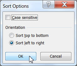
Clicking this button displays the Sort Options window which consists of only two options.  The first option lets you decide whether you want to sort with a Case Sensitive order.  Most people do not so this checkbox is not selected by default.  However, if you ever need to sort text data in which case matters, here is where you can adjust your sort.  The second option lets you select the sort orientation.  Normally, the orientation is set to top to bottom for sorting rows.  But to sort by columns, you must change the sort orientation to left to right.

 

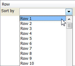
With the sort orientation changed, click OK to return to the Sort dialog and open the Sort By drop down.  Rather than display column names as you may be used to seeing, you will see row numbers.  Since our temporary row in which we defined our desired sort order was in row 1, we would select that option from the dropdown menu.

 

Continuing in the Sort dialog, you would probably still sort on values, but you may want to change the Sort Order to ready Smallest to Largest if it is not already set since we want the first column to be on the far left. 

 

When we press OK, Excel almost instantly redefines the column order based on our numbers as shown in the next figure.                                                                                                                             

 

Now the only thing left to do is to select Row 1 and right click on the row number along the left side of the screen.  Select Delete from the menu.  For sorting a large number of columns before importing them into SharePoint or any other system, this method is by far faster than manually dragging and dropping columns or even cutting and pasting.

Hope this saves your some time.