Fixing Color Contrast Issues

One of the more common compliance issues with ADA (Americans with Disabilities Act) is also one of the easiest to fix. Color contrast in relation to the text on the background requires that the text be easy to read by all users who access your website visually. Color contrast measures the difference between the font color and the background color on which the font is placed. The rule is quite simple:

1. Text consisting of a font that is greater than 14 pt bold (19 px) or 18 pt normal (24 px) must have a 3:1 contrast ratio with the background on which the font is displayed.
2. All other smaller text must have a contrast ratio of 4.5:1.

How do you calculate the color contrast between your font text and its background? You don’t need to know how to perform the calculation. There is a free tool that you can download and keep open on your desktop at all times so you can check the color contrast of everything you create. It was created by The Paciello Group and can be downloaded from this URL: The Paciello Group website – Colour Contrast Analyser.

But if the color contrast is not sufficient, how do you fix it. Well, of course, you try randomly selecting different colors, shades, hues, or tints of the original color until this tool calculates a satisfactory contrast ratio. For example, suppose the Colour Contrast Analyser was looking at a light blue (Hex: #1AB4E7) font on a white background (see image below). The initial colour contrast ratio is 2.4:1 which is too low even if the text was larger. You might think that the light blue on white looks good to you. However, you are not everybody and some people have more difficulty with colors than others. Thus, the Americans with Disabilities Act had to create a set of rules that were testable and verifiable to ensure a contrast that most people would find the resulting text to be easy to read against the background.

One way to ‘fix’ the problem is the click the dropdown arrow to the right of the box that displays the color which opens a grid of different colors as well as several different tints (adding white) to the base color and shades (adding black) to the base color. Because we want to increase the color contrast, we would perhaps try some of the shades. In the image below, the mouse is pointing to the second shade in the second (‘Shades’) row which has a hex value of #1487AE.

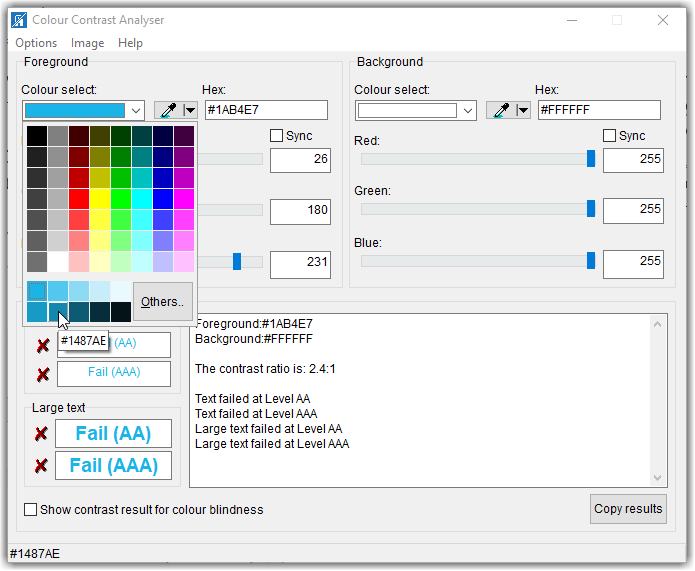
However, even this shade of blue is not dark enough to contrast with the white background resulting in a value of 4.1:1. Good enough for larger text, but if the text is smaller, it still falls below the 4.5:1 requirement. We could go back to select the middle box (#0D5A74) which results in a great contrast of 7.7:1. However, it may be too dark. I am not going to go through the trial-and-error steps here of going back and forth between lighter tints and darker shades until you find one that just satisfies the 4.5:1 rule without deviating too much from your original color. Rather, I am going to introduce you to a second tool that can help you find a satisfactory color without all that trial and error.

The tool that I found is called the Tanaguru Contrast Finder. This tool, while free, is not something you need to download. Rather just go to the Tanaguru home page for the contrast finder.

Open the Tanaguru site to use the Contrast Finder tool

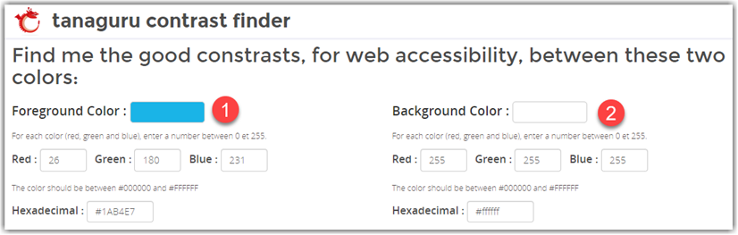
This tool’s home page lets start by specifying both the initial foreground (1) and background (2) colors. You can specify these colors either using the decimal values of the RBG color definition or you can enter the hex value of the color

Next, you can select the minimum colour contrast ratio you must meet (3). If the text is smaller, select 4.5 as shown below. For larger text, select 3.1

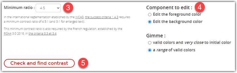
You can then select which color you want to change (4). In the case of regular text on the web page, you generally want to keep the page background color consistent across all of your pages. Therefore, I would change to the Edit the foreground color option.

You can also ask for colors that are very close to the initial color or a range of valid colors(4). I would in most cases go with a valid color very close to the initial color unless the contrast is too far from the ideal value in which case, I might ask for a range of valid colors to pick from.

When all the settings (1-4) are complete, click the Check and find contrast button (5). This is where the magic occurs.

After clicking the Check and find contrast button, the bottom half of the page is filled with possible colors that meet or exceed the color contrast you selected.

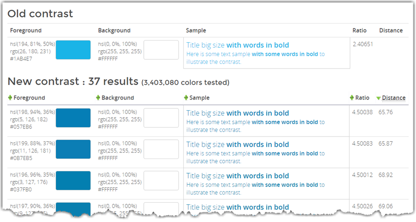
First, it shows the original foreground and background colors to give you a reference. To the right, there is a sample of the text so you can see what it would look like on a web page followed by the calculated contrast ratio.

Beneath the original colors, you see the possible colors the algorithm has selected. Even if they all look a little similar to you, the actual RGB values displayed in the leftmost column show that these really are different shades of blue. Note that the ratio column shows a calculated ratio of 4.5 or greater for each of the color combinations.

What I find instructive in training your eye to spot questionable color contrast text is to focus on the sample text from about 4-5 feet away. No matter how good your vision may be, you will often see a significant difference between the original colors and the selected colors, especially in this case.

Another example is the following image fragment from a web page I ran across. The first thing that my eye picked up was the green text on the white background. Indeed, this combination is only 2.5:1. However, not as obvious to most web page editors is that the red used in this table also has a low contrast to the white background. While it is better than the green, it still is only 4.0:1 which is below the required color contrast ratio of 4.5:1.

In fact, this shade of red is often picked out of a grid of colors as shown in the font color grid within the editor. As shown below, a pure red that also has the RGB value of (255,0,0) may seem at first to be a good choice because it may appear to be a bright red on a white background. Note, however, that bright colors often have poor contrast on a white background but may work fine on a dark background. Keep this in mind: the color selection dialogs in almost all cases have no idea what the background color will be. Therefore, it displays a range of colors, some of which may work with your background color, and many that will not. It is your responsibility to determine if the resulting color contrast with the background color is acceptable.

In this case, the darker red to the left (#C00000 or RGB(192,0,0) actually provides a good contrast with white resulting in a contrast ratio of 6.5:1. Don’t even get me started on orange on white or even worse, yellow text on white

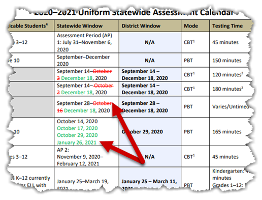
When you have text on a colored background such as the image shown below, the situation is much more complex because you can tweak both the font color and the background color to achieve the desired contrast ratio. (Yes, even text in images must meet the color contrast rules stated previously.) In this image, the yellow on the blue text has a ratio of only 2.1:1, the white font on a blue background is a ratio of only 2.4:1, the blue text on beige is only 2.2:1, and the red-orange on beige is a mere 1.6:1. I’m not even going to get into the effect on the crispness of the text when the image size is changed as was done here.

In a case like this, if you have access to the original graphic and can change the colors before you post the image, you must do that. Even if the image comes from a third party as is probably the case in this image, you cannot pass responsibility back to the third-party and use the image anyway. Either they must supply an image that satisfies ADA guidelines, or it cannot be used on your site.

Furthermore, this image contains substantial text that the vision impaired using a screen reader will not be able to ‘read’. Therefore, the text must either appear in the alt-text of the image or if there is too much text there (generally alt-text should be less than 160 characters), then the text should be elsewhere on the page or on a separate page linked from the ‘longdesc’ field of the image. In this case, to ensure ADA compliance, I would probably not use the image and just enter the text manually in a content portlet for the page.

In general, when looking at your page, you must consider people with all types of accessibility challenges such as:

• Visitors with low color contrast vision.
• Visitors who use screen readers to read the page contents.
• Visitors who have low hearing ability should your page use sound or voice.
• Visitors who cannot use a mouse to navigate around the page.
• Visitors who are affected by flickering images from animated gifs.

Putting yourself ‘inside the heads’ of all of these different visitor types is a challenge, no doubt. However, it is what is required of an accessible web page.

One last point, all of the above applies not only to websites but to any content you make available to others within or outside of your organization because you just don’t know what challenges they may face.  It simply is the right thing to do.

Tale of the alt, title and longdesc Attributes

Most of you probably know that the alt attribute found in the <img> tag is used by screen readers to assist the visually impaired and blind. What is alt text in the first place? It is the text that appears in place of the image if the user turns off graphics or if the user is using a screen reader as is the case for blind or visually impaired visitors to your site.

Is alt text always needed? Well the answer to that question begins with the question whether the image adds to the understanding of the other content on the page. As an example, look at this image found at the top of a page describing an art course:

Or even the following image found in the page header of an elementary school.

Do either of these images add any additional understanding of the art class page or the elementary school page? Would a user who turned off graphics or was blind or visually impaired and could not see these images really understand the rest of the page any less if they never knew the images existed? I would argue that they would not miss a thing. Therefore, these images are considered to be a decorative element on their respective pages and the alt attribute should be set to the null string as in the following: (not the word null)

alt=""

In addition, the title attribute should not be included for decorative images while it usually has the same text as the alt attribute. Strictly speaking, the title attribute is what the page visitor sees when they hover over the image with their mouse while the alt attribute is used by many search engines to catalog the image. So, having both of these attributes set to the same text is really not a bad thing.

Consider the following image with no text. How does it support the other content on the page?

In this case, you might have the alt text:

alt="Student races the car he built in the Engineering Magnet program."

Does it matter that the car is blue, the grass is green, they are on an athletic track, or that the student is wearing a helmet? Depending on the purpose of the story, the alt text shown above may be enough when combined with other content on the page.

On the other hand, suppose the image contains text as in the following image:

While the image itself may not add to the understanding of the content on the page, the text must be included at a minimum in the alt attribute as in:

alt="Physical Education"

Note that the alt text must convey the same information as the text in the image. It is not necessary to say that it is the “Physical Education Banner” or “Physical Education Logo”. Adding words like “banner”, “logo”, “picture” or “image” is considered superfluous.

Some images have text that must be repeated in the alt attribute such as for the following image:

alt="A blue T-shirt that says: We're all in this together".

On the other hand, names on the sides of buildings, text in store windows, etc. if not pertinent to the content of the page do not have to be mentioned.

Sometimes the alt text can even be simplified. It is not always necessary to repeat the image text word for word as long as the meaning and intent are the same such as in the following image.

alt="Click image for information about distance learning for parents"

Also, it is acceptable to convert the text to upper and lower case, define TLA (three-letter acronyms) as long as the converted text does not change the fundamental message of the image text.

What if the image and the text on the image do add substantially to the understanding of the page or even the purpose of the image. Then that information must be provided to the visually impaired in some way. If the image description is short or if the text is short, as we saw above, then the alt text can provide that additional information easily. But what if it is not short? While there is no physical limit on the length of alt text, it is recommended that alt text is kept short, 125 characters or less. Is that really enough to describe the image and the text on it? Take a look at the following image.

Repeating all of this information in the alt attribute with only 125 characters or less would be impossible. This was the intended purpose of the longdesc attribute.

However, contrary to popular belief, the longdesc attribute is NOT a place for directly entering longer text, perhaps paragraphs or more in which to explain the image or the text on it. Rather, the longdesc defines a URL where the visitor can get more information about the image and/or the text on the image. While the status of the longdesc attribute is not entirely clear under HTML5, the main point is that it is not a duplicate of the alt attribute text nor is it a more detailed explanation of the image even though longdesc sounds like long description. It is a reference to a bookmark on the page or to the relative or absolute URL address of another page that describes the content and/or text in more detail.

In the above example, we might have the text of this information repeated elsewhere on the current page. If so, we can identify the content section by adding an id attribute inside any one of the following content tags that precede the content:

<p id="GraduationEventTimes">

<h3 id="GraduationEventTimes">

<div id="GraduationEventTimes">

(Note: Each id value can only appear once on a page. Otherwise, how would a link know which location to branch to. Make sense?)

Then in the longdesc attribute of the image, we would include the following:

longdesc="#GraduationEventTimes"

Note that the name assigned to the id attribute can contain only upper and lower case letters, no space, no numbers, and no special characters. When the id is referenced, it must begin with the ‘#’ sign to identify it as a bookmark name and not a page name.

It is also possible to reference another HTML page found at the same level as the page with the image. Suppose this page was given the name: “GraduationEventTimes.html” or “GraduationEventTimes.asp”. Then the longdesc attribute would be:

Longdesc="GraduationEventTimes.html"

Note the absence of the ‘#’ symbol, in this case, to identify the relative reference URL as another page on the same folder level as the current page.

You can also use relative URL references to traverse your folder structure, but that is a more advanced topic than what I wanted to cover here.

It is even possible to reference a page using an absolute reference that might exist on an entirely different site such as:

Longdesc="https://myschoolsite.edu/Seniors/GraduationEvents.hyml"

Relative and absolute references are actually the preferred way to handle charts and graphs in which the longdesc attribute points to a ‘hidden from menu’ page that describes the data used to create the charts and graphs and perhaps even includes the actual data tables used by them. Obviously, that much information would never fit within the limits of the alt attribute.

Anyway, I hope you learned something here about the alt, title, and longdesc attributes found in the <img> tag and to not use the longdesc attribute just to insert additional text describing the image or text in the image.

Working with Themes – Part 8

In Part 1 of this series, you learned how to use some of Power BI’s built-in.   

In Part 2 you learned about Microsoft’s Theme Gallery.    

In Part 3, you learned how to use the new Customize the Current Theme. 

In Part 4, you learned how to export your customized theme and to use it in your future Power BI report projects.   

In Part 5, you learned how to create a simple JSON theme file for your future Power BI report projects.  

In part 6, you learned about a few of the more common attributes used to customize the color of elements in the most commonly downloaded visualizations.

In part 7, you learned about a few more generic classes that define the colors for conditional formatting and KPIs.

By now you have seen several cases where the colors of some elements would change ‘magically’ when you apply a new theme to your reports. This is part of the artificial intelligence behind Power BI that looks at the color changes that have been applied by a theme and attempts to ‘adjust’ colors of other elements that have not been specified by the theme to something that should be compatible. If you remember, I touched on the fact that background colors appeared to change with some themes that defined only the dataColors array, but then was able to modify the background color by specifically using the background class. However, supplying a background class color also appeared to change the colors of other elements. I will not pretend to understand how that is done by Power BI so I am going to remind everyone of Arthur C. Clarke’s quote from “Profiles of the Future”: “Any sufficiently advanced technology is indistinguishable from magic.” However, if you can wrap your head around a hierarchy of color elements in which Power BI generates default values only if you do not define the color of those elements directly, you are on the right track to understanding how to control your theme colors.

That being said, as we dive further into the capabilities of JSON defined themes, we find additional ways to define those deeper elements which previously Power BI generated colors for when we did not specify them in our themes.

This week, I want to look at what Microsoft calls structural colors. Every visualization has some sort of structural element. These are typically elements outside of the typical data elements that are being displayed. They have been divided into first through fourth level elements. There is also a class for general background and for secondary background colors as well as Table Accent colors which is basically the grid outline.

Here is the problem, or challenge depending on how you look at it. How do you remember which structural elements appear in which of these 7 color classes? Honestly, I have not found an easy answer to this question other than to keep handy the table supplied by Microsoft (found in the How to Create a Theme link at the bottom of the ViewàThemes dropdown menu) and displayed below.

When you look at the table, notice that several class names have (deprecated) after the name. This does not mean that the entire class has been deprecated. Rather only an old name for the class has been deprecated. For example, the class name ‘foreground’ has been deprecated and is now known as ‘firstLevelElements’. Perhaps a comma between the new and old class names would have helped clarify that. Therefore, in my table below, I’ve added those commas. I’ve also added commas in the right column to help clarify what structural elements each color class formats.

As mentioned above, you should also note that we have seen three of these color classes before when we used the class names: background, foreground, and tableAccent. In fact, these three color classes appear in many of the themes that you can download from the Theme Gallery. They are used to provide compatible colors for many of the structure elements when using these themes. However, the class ‘foreground’ is being deprecated and should be replaced going forward with ‘firstLevelElements’. While both class names will work at the time of this writing, it is something that you should be aware of because someday the ‘foreground’ class will no longer be accepted when loading a theme. I am hoping that this will not affect older reports that previously applied themes with the deprecated class names. However, I have no secret insight on that question.

In the following table, you can see 7 color classes

Color class	What it formats
firstLevelElements, foreground (deprecated)	Labels background color (when outside data points), Trend line color, Textbox default color, Table and matrix values and totals font colors, Data bars axis color, Card data labels, Gauge callout value color, KPI goal color, KPI text color, Slicer item color (when in focus mode), Slicer dropdown item font color, Slicer numeric input font color, Slicer header font color, Scatter chart ratio line color, Line chart forecast line color, Map leader line color, Filter pane and card text color,
secondLevelElements, foregroundNeutralSecondary (deprecated)	“light” secondary text classes, Label colors, Legend label color, Axis label color, Table and matrix header font color, Gauge target and target leader line color, KPI trend axis color, Slicer slider color, Slicer item font color, Slicer outline color, Line chart hover color, Multi-row card title color, Ribbon chart stroke color, Shape map border color, Button text font color, Button icon line color, Button outline color,
thirdLevelElements, backgroundLight (deprecated)	Axis gridline color, Table and matrix grid color, Slicer header background color (when in focus mode), Multi-row card outline color, Shape fill color, Gauge arc background color, Applied filter card background color,
fourthLevelElements, foregroundNeutralTertiary (deprecated)	legend dimmed color, Card category label color, Multi-row card category labels color, Mulit-row card bar color, Funnel chart conversion rate stroke color,
Background	Labels background color (when inside data points), Slicer dropdown items background color, Donut chart stroke color, Treemap stroke color, Combo chart background color, Button fill color, Filter pane and available filter card background color,
secondaryBackground, backgroundNeutral (deprecated)	Table and matrix grid outline color, Shape map default color, Ribbon chart ribbon fill color (when match series option is turned off),
tableAccent	Overrides table and matrix grid outline color when present

So, suppose we created the following theme. Yes, this is still a theme even though we did not define values for the dataColors array element.

If you did not get what you wanted or expected when you applied this theme, maybe you need to combine everything we learned so far into a more complete theme definition such as:

Anyway, I leave you to ‘play’ with what you have learned so far to see what new themes you can come up. In any case, we have not reached the bottom of this deep dive into themes yet. Stay tuned. Next time I will show you how to manipulate text families, colors, and sizes.

This Saturday, I will be speaking at SQL Saturday, Tampa on this theme, so to speak. If you are planning on attending, stop by my afternoon session or look for me to say, “Hi!”

Working with Themes – Part 4

In Part 1 of this series, you learned how to use some of Power BI’s built-in themes to change the color themes of your reports. This of course was better than having to manually customize all the elements in your visualizations, but you were limited in the number of themes available.

In Part 2 you learned about Microsoft’s Theme Gallery where 3^rd party developers have offered their custom themes, mostly for free, to anyone who wanted to use them. Yes, you had to go through a few more steps, but this opened the doors to dozens of new themes that you could use to add different colors to your reports.

In Part 3, you learned how to use the new Customize the Current Theme feature that was added as a preview feature in December 2019. One of the great things about this feature is that it allows you to start from any theme and customize it to look exactly the way you want. But that is just part of the benefit of customizing a theme.  The rest is what I’ll talk about today.

Exporting Your Customized Theme 

In the ancient past, as in a few months ago, if you wanted to theme all of your Power BI reports the same way, you not only had to manually set all of the color and text attributes for every visualization in a report, but you had to write down those settings so that on the next report you could configure the colors and text attributes the same way. While that was certainly doable, it was usually not worth the time and effort. A few users may have figured out enough of the JSON coding of themes to create their own custom theme and use it in each of the subsequent Power BI Report files. We will talk more about that method next time and why that might be your preferred option.

However, with the ‘Customize the Current Theme’ feature, you can start with an existing theme from the Theme Gallery that is close to what you want and customize it one time and then reuse it and even share it. That’s right. One time! Because with the addition of the Customize the Current Theme feature, you also have the ability to export the theme from your current Power BI file and save it as a JSON file.  You can then import this JSON file using the ‘Browse for themes’ option just like any other theme file you may have downloaded from the Theme Gallery we talked about in Part 2.   

 

You just have to give your new theme a unique name (remember that was on the first panel of the Customize the Current Theme dialog). You can save the theme file anywhere, but I personally like to keep a single folder on my hard-drive that holds both my downloaded and my customized themes.

Making your Customized Theme a Standard 

Once you create a theme that is branded to your own personal tastes, your school or college colors, your corporate or organization’s color palette or for any other reason you need a special theme, you can save that theme definition as a file and share it with others. If everyone loads that theme into their report, then all report visualizations will look like they are all from the same person or part of one branded organization no matter who creates them.

One way to achieve consistency in branding is of course to share the exported theme to everyone so that they can import it into each Power BI file they create. However, this method could be problematic because some Power BI Users may not load that theme into their reports and proceed with either a different theme or with manually customized colors and fonts. Unfortunately, there is currently no way to change the default theme within Power BI. Maybe that feature will be a future enhancement.  In the meantime, one way to make compliance easier is to open a new but empty Power BI file, one in which no data has been loaded yet. Next, open View -> Themes and browse for and open a saved theme. Then save the empty Power BI file without adding any data to it. Then when you or anyone else begins a new Power BI file, start with this saved branded file to start a new report. For example, I save an empty Power BI file with my preferred theme using the name default.pbix. If I start a new report with this file, I will automatically have the same theme I used in my other Power BI files.

If you follow the suggestions above you can achieve a consistent look and feel across all of your Power BI reports. When used at a department, corporate, or organization level, it lends an air of professional branding to your work rather than the appearance that everyone if off working on their own.

What To Do When a Custom Theme Appears Not To Work 

Normally, when you apply one custom theme on top of another custom theme, the new theme replaces all the colors and fonts of the old theme (unless it is such an old theme or one that only defined a limited subset of the elements it would customize). Sometimes when you attempt to brand a previously created Power BI report, the branding colors or fonts do not appear to work, or perhaps they work on some visualizations but not on others.  Does this mean that there is something wrong with your branding? Probably not. It merely means that the default color or font used on one or more visualization was manually changed prior to applying the theme. Theme changes will not overwrite manually set branding. I suppose this is a good thing because the assumption is that you set those branding changes on purpose and you would not want to lose them due to applying a different custom theme to the rest of the report.

But what if you really wanted the branding of the custom theme to apply everywhere with no exceptions. Well, I suppose you could start over with the desired theme loaded first before loading data and creating visualizations. However, that would require a lot of work. Another way to fix this problem is to go into the formatting of each visualization and revert the branding to the default. Then reapply the desired custom theme.  That is still potentially a lot of work, but not as much as starting all over.

To revert the formatting of a visualization to the default, you do not have to remember the original colors, fonts, or font sizes. That would still be considered a manual customization.  Rather, you can select the visualization and open the Format panel. Expand each section within the Format panel and look for the text ‘Revert to default’ at the bottom of the section. Note that not all format sections may have or need this option.   

 

Even if you manually changed the color to other colors taken from the prior theme using the theme’s color palette, you will need to revert these colors and fonts to their original settings before a new theme will replace them.

Well that is all for this time. Next time, we will begin a dive into creating JSON files directly. Why would you want to do this?  Afterall, now with the ability to customize themes using a dialog, defining your own theme is simple and easy.  Well, you will have to come back next week to see if building a theme from scratch is right for you.

C’ya. 

Calculating Percentages in PowerBI

Last time I showed how you can pivot a multivalued column from a survey downloaded from SharePoint to Excel. After some transformations, I created the following report that shows the number of career responses in each of the 18 categories. While interesting in of itself, it would be more interesting to see how the career choices break down by different dimensions such as the school or grade level, the gender of the student, or perhaps even by individual school.

In my report page, I am going to reserve an area along the left side of the page to list several of the dimensions I’m interest in and to display the total number of students that took the survey along with the number of students in the filtered subset when I filter by one of the dimensions. Basically that means building something like the following:

This image actually consist of four separate visualizations. The top visualization for Total Students uses the Card visualization and initially displays the count of the ID column in the survey table that has one record for each survey. I duplicate this visualization and drag it below the first one. Then for the top visualization, I open the Format option panel in the visualization section and make the following changes:

• I turn off the Category Label
• I turn on the Title and then open the Title section to add the Title Text: Total Students
• I change the font size and color to make this information stand out.

I then repeat the process for the second visualization but with the Title Text: Sampled Students because this count will represent the number of students included in the visualizations taking into account any filters applied to the page.

I then add two single column tables, one for gender and one for grade level. Because I want to use the values in these table as page filters, I change the visualization of these two tables to the Slicer.

Along with the table I created in my last blog, I can work with the slicer values to explore how the career choices change based on gender and grade level by clicking on the check boxes. When I do this, I see that the chart automatically adjusts the columns based on the changes I make to the slicers. Also the number of sampled students in the second card visualization displays the count of students included after applying the slicer. Unfortunately, the total student count also changes. This I do not want. I want the total number of students to always represent all the students in the entire survey.

I can achieve this goal with a little DAX and a custom measure back in the data page for the survey table. The custom measure needs to count the IDs for all the records in the table ignoring any filters applied to the report page. I can do this by passing the survey table name to the ALL() function. This function ignores all other page filters. Then I use the COUNTAX() function which defines the data source as the output from the ALL() function and then performs a count the number of IDs. While this may sound complicated, it is as simple as the following equation:

Notice that I name the measure Students. I must provide a unique measure name for each measure I create. However, I can then use that measure in any visualization such as the card visualization for the total students in the survey.

Back on my report page, I select the top card visualization (for Total Students) and change the field used from ID to my new measure, Students.

Now if I select any of the values in the slicer visualizations, my sampled students card displays the number students included in the filter while the total students card displays the total number of student surveys taken as shown below.

I then add on the right some additional column visualizations to display other data fields such as which subject the student finds most interesting in school or charts that display career choices by gender, by grade level or by other criteria from the survey. Each of these charts begins with a simple table visualization in which I add the columns I want to use. I then convert the visualization to a column chart.

In the image below, you see the final result of the first page of my report. Notice that I also added a vertical line shape to separate the two card visualizations and the slicers from the other column charts.

Since each student was allowed to select one or more careers from the list of possible careers, the total number of career choices is significantly larger than the number of students. In the above figure, the count of career interests, if I were to add the values in each of the columns, would total the number of career selections which is over 17,000, not the number of students. Therefore, I might decide to display the same charts as a percent of all the students rather than a count of all career selections.

Again I need another custom measure to calculate the percent based on total students. Fortunately, I already have a measure that calculates the total student count ignoring any slicer selection or page filter. Therefore, I can generate a percentage using a formula similar to the following:

With this formula, I count the number of surveys filtered by the visualizations and slicers on the page divided by the total number of students who took the survey. The maximum value of this percentage would be 100% if all the students who took the survey selected the same career, such as computers, as one of their choices. Similarly, the minimum value would be 0% if no student selected a specific career as one of their choices. Because students could select more than one career of interest, the sum of the percentages of each of the columns will not add up to 100%, but some value greater than 100%. (Lesson learned: Next time ask for their preferred career choice, then their second career choice and finally their third career choice.)

Next I take the first page of my report and duplicate it by right clicking on the page tab and selecting the option to duplicate the page. (This is a lot faster than recreating the same visualizations on a new page, isn’t it?) On the duplicated page, I modify each of the column charts to display the Percent measure just created rather than the count of ID.

Why does this work? Well, because each student can only select any specific career one time even though they may select two, three, or more careers, I can simply count the number of filtered students in each column by the total number of students in the survey. Each chart already divides the students by career choice, one career for each column. Then additional filters from the slicers may limit the gender or grade level or both. Therefore, I can count students that match all those filter criteria and divide by the total student count to get a percentage of students who have an interest in that career. In fact, this measure also correctly calculates the percent of students interested in each school subject (of which they can only select one subject each) which I can verify by summing these percentages from the chart in the upper left and getting a total of 100%.

The following figure shows the percent page of my report.

I can then proceed to add other visualizations if I want on additional pages. But I’ll suspend this example at this point for now.

C’ya next time for more exciting ways to use Power BI.

The Need To UnPivot Data

Today I am going to take a look at some interesting issues I encountered when pulling data from a survey into Power BI to perform some analysis. First some background. The survey existed on our SharePoint site and all submissions were stored within SharePoint. However, as a list, it is always possible to download the details from the survey to an Excel file. When I open the resulting Excel file, I see the following data.

Most of the columns are straight forward text columns. But, looking closely at the rightmost column I see that the data structure is a bit more complex than usual. This is the result of having a survey question in which the respondent is allowed to select one or more items from the list of possible careers that they have an interest in. While some may only respond with a single career that they are focusing on, others may not be so sure yet and so they have selected multiple careers in which they may have an interest.

You can see that the format of the data consists of responses along with the corresponding ID values of the selected responses separated by semi-colons.

Obviously, I cannot perform analysis on such a column with multiple values. I need to get this data into a single vertical column with one row for each career choice selected by the respondent. The first step to achieve this result is to split the individual career values into separate columns. I can do this in Excel by selecting the column with the multiple values and then selecting the button: Text to Columns in the Data ribbon. This function allows me to split the text in each cell of the column into multiple columns each time a specific delimiter is found. In this case, I can split the original text at each semi-colon to create a new column.

After splitting the data into columns, there are some column that I no longer need and can delete. These are the columns that contain the ID values of the selected career values. I have no need for the ID values. I can also apply a series of Replace statements to clean up the rest of the career values to remove extra characters that are not part of the career name itself. After a few transformations, I’m left with the following set of spreadsheet columns which identify the respondent with their ID and then the careers in which they have an interest.

This is still not exactly what I want because I really need to normalize this structure to get multiple rows for each responder with one career choice per row. However, as I will show in a moment, I can perform that transformation in Power BI much easier than it can be done in Excel. So let me proceed to open Power BI and select Get Data.

When I open Power BI and choose Get Data, I select the Excel data type and click the Connect button. In the next screen (not shown) I will either enter the path to the Excel file or I can browse to the file using the Browse button. Once I select the Excel file I want to work with, Power BI opens the file and displays all the tables found in that file. In the figure below, you can see that there are several tables. Some of these tables consist of the original raw data and the transformation steps I used to create the datasets that I want to work with. Each table corresponds to a different tab in the Excel workbook otherwise known as an Excel Worksheet or simply Sheet.

After selecting the tables I want to work with, I click the Load button to import the data into my Power BI model. Some transformations might be needed to ‘convert’ some of the columns to user-friendly data names. I could have also done this in Excel by changing the column header text. However, the transformation I want to focus on is the career choice table which I call PreCareers. A portion of this table appears below. This table consists of the ID column used to identify the responder along with 18 columns representing their potential career choices. While most respondents only entered three or less career choices, some entered significantly more. By default, the data is sorted with all respondents who had only a single career choice displayed first. Those are followed by the respondents who selected two career choices and so on.

In order to create a table that has the ID of the responder and a separate row for each career choice they selected, I need to unpivot the 18 career choice columns. To do that I need to select the Edit Queries button in the Power BI Home ribbon and then select the PreCareers table. Next I have to select all 18 career choice columns. Then opening the Transform ribbon, I look for and select the Unpivot Columns command as shown in the following figure.

After selecting this option, Power BI performs the transformation to create a new table shown below which now has a column that has the previous column headers in a column named Attribute and a column named Values that contains the career choices. Of course I can rename these columns and probably will, but let save our work as a safety precaution before continuing.

To save my changes, I would select the Close and Apply button from the Home ribbon. Remember that I can save my transformations multiple times and return back to Edit Queries to insert additional transformations at a later time.

However when I attempt to close and apply my changes, I get the following error message.

Reading this error message I see that there is a problem with the Column ID in my transformed PreCareers table. If I open the tables in diagram view mode as shown below, the problem is evident.

You can see that the PreCareers table is linked to the K8_Survey table using a 1-to-1 relationship which if I were to look at the relationship is attempting to connect the ID column from one table to the ID column of the other table. The problem is that now that I unpivoted the selected careers in the PreCareers table, there are now multiple records with the same ID value, not just one record.

To solve this problem, I must remove the current relationship as by right clicking on the relationship and selecting Delete as shown in the following figure.

You may have also noticed a yellow bar across top of the page, shown below, that says that there are pending changes to your queries that have not been applied. With the relationship deleted, I can try to apply the changes again by click on the Apply Changes button.

As the changes apply, I see that the field names in the PreCareers table are updated as are the field names in GradeLevel table.

I can now use drag and drop to create new relationships between the tables. For example, I can click and drag the ID field from PreCareers table to the K8_Survey table as shown below. I can also connect the School field in GradeLevel with School in K8_Survey relating these two tables.

With the relationships on my restructured tables back in place, I can go to the Report page and begin to create a report table that displays the possible career choices along with a count of the number of times that career choice was selected.

With a simple change of the Visualization from a table to a column chart, I can visually show which careers were selected the most by the respondents. Note that because each respondent can select any number of careers and they can be selected in any particular order, there is no way to reliably rank the career preferences to say one career or another is truly the top career choice. The chart can only say which career choice was selected the most often of all careers the respondents had an interest.

Another important point to remember here is that the sum of the number of times each career choice was selected is NOT equal to the number of respondents because any respondent could select any number of career choices. Therefore if you want to know the percent of respondents who selected computers as a potential career, you need to know the total number of respondents, not the total number of responses.

I’ll delve more into the analysis of this data next time, so save this file.

BTW, this weekend I am at the Orlando Code Camp held at Seminole State College in Sanford, FL. If you happen to attend, please stop by to say hello. I’ll be conducting two BI related sessions, one for Power Pivot and one for Power BI.

C’ya.

An Aster Plot for the Holidays

Yesterday was Christmas and for those who celebrate Christmas, I hope you had a very happy day. However, I just wanted to ask this. Why do we wait for Christmas to be nice to one another, to wish our fellow man peace on earth and goodwill to all men? And do we really mean it or do we just go back to our old ways the day after. Do we need a holiday to be nice to each other? Why cannot the Christmas spirit spread throughout the year? And why does it have to be tied to a religious holiday. Do we need a religious holiday to tell us when to be nice to others?

On a similar note, New Year’s resolutions are coming up in another week. Could we all possibly resolve to act a little more like Christmas every day of the year? Or is that just as hard as resolving to lose weight?

Anyway, since many of you are on vacation anyway this week, I’m going to do just a short blog on the Aster Plot visualization for Power BI. This visualization, like many of the others I’ve talked about can be found on Microsoft’s Power BI Visualization Gallery page. When you click on the Aster Plot tile, the following diagram displays telling you a little about the visualization which as they state in the description is related to a donut chart. However, unlike a donut chart which defines the size of the donut segment on the value associated with that segment much like a pie chart, an aster plot uses one dimension to define the segments and each segment is equal in the amount of the arc it uses. The value associated with the segment defines the radius of the segment instead. Let’s see how this might work with some of the sales data by product category from Contoso.

I’m not going to go through all the dialogs that appear when you download a new visualization. I’ve done that before. So if you are joining in for the first time, check back through some of my previous blogs for details on that.

After the visualization is downloaded, I can load it into my Visualizations toolset/panel by clicking the ellipsis (3 dots) at the bottom of the visualizations panel.

Power BI will display a warning to caution you about importing custom visualization, so you should always do this on a test machine first to make sure they do not cause any issues. Just because it is on a Microsoft page does not mean that it is safe to use and does not violate any privacy concerns.

Next, I loaded my Contoso data and displayed the Sales Amount by Product Category as shown in the table below. (Again, if you do not know how to do this is Power BI, I’ve covered this several times in the past several months.) I should mention that I specifically sorted the sales data in descending order for this visualization.

Then with my table selected, I can click on my new visualization, the Aster Plot which displays the chart shown below.

Notice that if I hover over any of the segments, a box appears that tells me the product category name along with the corresponding sales amount for that category. One of the things that I don’t particularly care for is that the name of the dimension appears in the center of the chart and apparently behind the arcs so some that some of the name is covered by the chart. I wish I could move the dimension name either to the top of the bottom of the chart at the very least. Of course I could customize the name to make it smaller or to add spaces between the words back on the data page, but for this demonstration, I didn’t feel the need.

You can have other charts on the same page like the one shown here that displays the Sales Amounts by calendar year for Contoso.

Like other visualizations, I can click on any of the Aster plot segments to select that category and the column chart to the right will automatically update to highlight the annual sale for the selected category while still showing in a lighter shade of the column color to total annual sales.

Similarly, I can select a year and the Aster plot will be redrawn to display the relative sizes of each of the categories as shown below.

Well, that is all I’m going to cover for this week because it is time to get back to end-of-year celebrations, visiting relatives, after-Christmas sales, and all those things.

C’ya next year.

Power BI – Measures and Slicers

Sorry about missing last week but it was a holiday here in the states where parents encourage their kids to go up to strangers and ask for candy. Also people of all ages, not just kids, get dressed up in costumes that range from the cute Elsa princesses to the DBA zombies and the slutty managers. Yeah, some of them were really scary especially since it wasn’t always a costume.

Anyway, last time I talked about creating custom columns and added the column TotalProfit to the FactSales table of my model. (If you missed that discussion, go back to my blog from two weeks ago.) Column expressions are easy to create because they largely resemble row context expressions that you might add to an Excel spreadsheet. In fact, most of the syntax and functions are exactly the same as in Excel.

But we can also add custom measures. The difference between a column and a measure is that most columns can be used as dimensions in a pivot or matrix table especially the columns that contain alphanumeric data. Typically the columns that have numeric data appear as aggregated values, summed, averaged, minimized or maximized depending on the goal and the dimensions used. In fact, the TotalProfit column, while calculated for each row in the FactSales table, is typically displayed as a summed value such as in the following image taken from where we left off last time.

In this matrix table, the TotalProfit is first calculated for each row in the FactSales table that will be included in the final matrix table, but the individual calculated values are then summed by one of five channels that exist for sales. Thus with my sample data, the calculation for TotalProfit occurs a little over 3 million times, but these calculations are made only when the column is created, not for each visualization. Then those values are summed by channel for the above visualization. As this happens on my Surface computer in less than a second, that is still pretty impressive. However, there is another way we can calculate total profit for this table.

We can create a measure to calculate total profit. A measure is calculated each time it is used in a table. In a table like the one above, a total profit measure would only be calculated four times, once for each channel, but each calculation would include three sums over potentially hundreds of thousands of rows and these calculations occur when the visualization is created and in each visualization the data might be needed. To create a measure, find and click on the New Measure button in the calculations group of the Modeling ribbon.

In the expression box, I can see the start of the expression. Note that unlike PowerPivot, the measure name is followed by just the equal sign rather than a colon and equal sign. The rest of the expression is similar to what I used before except that I have to aggregate (in this case sum) each of the values in the expression (you cannot sum an expression). In order to distinguish this expression from the prior one, I include an underscore between ‘total’ and ‘profit’.

After defining the measure, it appears in the field list on the right. While it is still selected, I go to the formatting section of the ribbon and adjust the data format to $ English (United States) which gives me comma separators and two decimal places by default. Note that I can and should do this for any other table field that I will use in a visualization.

Now I can add this measure to my matric table from above replacing the TotalProfit calculated column with the Total_Profit measure. In order to calculate the total profit for channel sales, Power BI has to sum the SalesAmount column for all channel sales and subtract from it the sum of channel total costs and the sum of channel discount amounts.

Your first thought might be to ask how is this better than calculating the total profit for each row in the FactSales table and then simply summing the included rows into a single value. Well like a lot of things in the real world, it depends. Typically a calculated column increases data load times each time you load the model because only the expression is saved, not the individual values (or at least so I’ve been led to believe), but for many visualizations that use most if not all of the data, the impact on calculating the values for the visualization are no worse and possibly even less than using a calculated measure. On the other hand, for a calculated measure that only appears in a few visualizations or when the visualization has been filtered to include a smaller subset of the total data, a calculated measure can improve both data load times and dashboard display times.

But perhaps more importantly, not all expressions can be written as either a calculated column or a measure interchangeably as I have done here. For example, if I wanted to calculate the percent that each channel sales represents from the total sales, I would have to use a measure because there is no way to aggregate percentages over multiple rows. I want you to think about that and I may return with a detailed example in a future week. In the meantime, I want to explore one additional feature of this model.

Those of you who have followed me through my travels in using PowerPivot remember the concept of using slicers to allow the user to analyze different segments of the data by clicking on dimension values. For example, using the above table, I might want to see the profit numbers for different product categories. In PowerPivot, I could create a slicer and if I had more than one visualization on a page, I could associate each chart or table with that slicer.

In PowerBi, I can also define slicers for the reports on the page. To do so, I click in a blank area and select the field from the dimension table that I want to use as the slicer/filter. In this example, I will use the ProductName field from the dimProductCategory table. This dimension only has eight values. The table is relatively short and appears initially as shown below.

To convert this table list into a slicer, I need to select the Slicer visualization as shown in the following figure while the above table has focus. This tells PowerBI to use the table as a slicer rather than just displaying the values of the field. (Yes, I could add a filter to the visualization directly, but a slicer can automatically apply to multiple visualizations on the page.)

After being defined as a slicer, each value of ProductCategoryName has a selection box to its immediate left and two additional entries have been added to the top of the list to select all values or to select only those records that have a blank for the product category.

If I click on any one of the categories, the data in the other visualizations on the same page automatically filters out all records from other categories as shown below.

I can also select multiple categories by clicking on several of the checkboxes to include in the matrix sales from all of the selected categories. Note that in a case like this, the measure I defined actually will perform fewer calculations because the sum function only acts on the filtered records of the slicer, not on all records in the channel.

I can return to displaying all categories either by clicking the Select All option, by clicking on each of the individual category names, or by using the Erase icon to the right of the table name.

C’ya next time.

Deriving Columns from What You Know in Power BI

Before I get started with the topic of the day, I want to remind you that Power BI is still being updated by Microsoft. In fact, there was an update just last week on October 20th that appears to have added some missing features that I mentioned before. So if you haven’t updated Power BI recently, be sure to do that before reading the rest of this blog.

A few weeks ago when I was looking at defining relations between tables in the Relationship dialog I was disappointed in the fact that when I display my tables in what I would have previously called a Dialog view in PowerPivot, I could not use drag and drop to define my relations. Well, my disappointment is over. The latest update, among other things, adds this capability.

Since last Wednesday, October 21, was ‘Back to the Future’ day, I want to go back to last week’s blog just after I added the DimProductCategory table. This time however, rather than using the Management Relationships dialog, I am just going to the Relationships view and drag the field ProductCategoryLabel to ProductCategoryKey as shown in the following image.

Now I must say that I am use to just identifying the fields from my two tables that I want to connect to form the relationship and expect PowerPivot to figure out which is the one and which is the many table. Unfortunately, Power Bi still is not quite this smart. Because when I attempt to define this relationship from the one site to the many side, the relationship definition fails as shown in the following figure.

Maybe the next update will automatically reverse the direction of the relationship for me. However, for now I can click the OK button in the message box shown above and then redefine the relationship correctly from the DimProductSubcategory to the DimProductCategory table.

Now the relation is created and I am ready to continue. By the way, when I click on the relationship, Power BI highlights the two tables as well as the relationship line. It also encloses the connecting fields in a box to make it easy to identify the relationship fields.

If instead of left clicking on the relationship, suppose I right click on the relationship. Now I get an expected option menu which in this case consists of only a single option, Delete. Clicking this option will of course delete the relationship.

On the other hand, double clicking on the relationship opens the Edit Relationship dialog shown below. I can use this dialog to view the relationship or a sampling of the data, or make changes to the relationship.

That’s great. But like an infomercial, there’s more! In the Relationship view (Diagram view) I can also now right click on a field and delete a field, hide a field from the Report view or rename the field.

As with PowerPivot, if I delete a field, it is gone for good. If I realize later that I need the field, I would need to delete the table and reload it to get the missing field. Of course there are other consequences to doing this like needing to redefine the relationships and possibly rebuilding reports (visualizations) that used that table. Because at this time, I cannot visually define the fields to include or exclude during my original data load from my data sources, it is important that I know my data and delete any fields that I know that I will not need before I begin creating new columns, measures, or reports. In PowerPivot, we called these columns Useless columns.

I can also hide some columns from the Report view. For example, I can often hide columns used to define relationships between tables because end users typically do not include these columns in reports. Hidden columns are referred to as Technical columns because they are required in the data model and cannot be deleted without destroying relationships or perhaps calculations of other fields. I never want to show more columns to a user than they know what to do with.

Finally, renaming columns can be very beneficial. Often column names in databases have cryptic or abbreviated names. End users may not be comfortable with these shorten names. Use the Rename feature to make names user-friendly and descriptive.

Not only can I delete, hide, or rename columns in a table, but by right clicking on the table header, I can perform these same actions on an entire table. For example, I may not like dimension tables that begin with the letters ‘Dim’ like many DBAs prefer but end users may have no idea why the table is Dim. Similar to columns, I don’t delete tables from my model unless I am positive that I do not need them. Hiding tables only makes sense if I want to use only one or two fields from a table. In this case, I may need a column from another table for a calculation, but I would never display those columns directly in reports.

Returning to the data view of my tables, I can also right click on any of the column headers and delete, hide or rename the column. There are also several other options ranging from sorting, to creating new columns or new measures.

I can also right click on the column names in the fields list along the right side of the Data view. The dropdown list of options shown below is similar to options in the context menu above. So I have several different ways to manage columns

Let’s try something new, a new column in fact. In my FactSales table, I can find several columns like SalesAmount, TotalCost, and several others, but there is not Total Profit column. I can easily calculate that value from other values in the table. To begin, I need to create a new column in my data model. That means clicking the New Column button in the Modeling ribbon.

New columns are created at the right end of the table. By default, the column name is cleverly called Column. Of course I can change that by entering a new name. Then after an equal sign which indicates that an expression will be used to define the column, I can begin entering the column definition using DAX expressions. Yes, DAX is still alive and well. If you need a review of using DAX, I’ve covered multiple DAX topics over the last couple of years of this blog.

As in PowerPivot, I can select a column from the current table by just typing the left square bracket. This action opens a dropdown of all column names in the current table listed alphabetically. I can scroll down through the list and select a column by double clicking on its name. I can also type a few characters of the column name to narrow down my list as shown below.

My full expression to calculate TotalProfit is shown below

When I click the Enter key, the entered expression is used to calculate the values for all the table rows.

Before moving off the column, I might want to define custom formatting for the values. The formatting definition here is carried forward to all reports generated with the data. In the above example, I might want to only display the dollar amounts to two decimal places. (Actually, because of the size of aggregated data, I might later decide to format the values with no decimal places.)

Suppose that I want to display some of this data using a standard table with Channel names for the rows and a few select columns from the table. Notice that the values displayed here obey the formatting definition set on the Data page.

That’s it for this week. Next time I cover creating New Measures and why you might want to do so.

C’ya.

Creating Relationships Manually in Power BI

Last time we loaded a BI model with data from several different data sources, but the data sources were carefully selected so that the columns that would relate one table to another table would already have the same name and data type before attempting to upload the data to Power BI Desktop. Because of this assumption, I was able to let Power BI auto detect the relations between the tables. Unfortunately, in the real world, that does not always happen. So this time I will show you how to create relationships manually and how you may need to massage the data a little first before defining those relationships.

I am going to use the Contoso data again and will begin with the following tables already loaded into the model from my SQL Server instance: FactSales, DimChannel, DimDate, DimProduct, and DimProductSubCategory. To complete my model, I need the Product Category data which I am going to load from an Access table in this case.

Since we covered how to load data from SQL Server last time, I am going to pick this discussion up after I have loaded the SQL data and am about to load the Product Category data. The image below shows that I have already click the Get Data button and have selected Access database from the list of possible data sources and have defined where my Access database could be found. As you can see in this figure, Power BI only finds a single table in my Access database named DimProductCategory. When I select this table, I see a preview of the data.

In the table preview (on the right), I see that there are only two columns named ProductCategoryLabel and ProductCategoryName. You might be able to guess from the way the data in the column is formatted that the ProductCategoryLabel data has been defined as text, not numbers because it is left justified.

After clicking the Load button to import this data into my data model, I switch to the relationships view and see the table diagram shown below.

I see that there is no relationship defined with the DimProductCategory table because there are no connecting lines leading into or from this table. Therefore, I first want to select the Manage Relationships button. I can see the four relationships that tie together the other five tables, but I am missing a relationship. I may first try to click the auto detect button which I talked about last time to see if Power BI can find the missing relationship

Unfortunately, Power BI very quickly responds back that it cannot. The problem is that while the DimProductSubcategory table has a field named ProductSubCategoryKey, the new table, DimProductCategory, does not have a field with that name.

So I might try to create the relationship manually by clicking the New button on the Manage Relationships screen (after closing the Autodetect message screen of course).

On this screen I have to specify the names of the tables and the linking columns to define the relationship. I can begin with either table on the top. After I select the table, I see a grid of the available fields along with a couple of rows of data. To select the field that I want to use in the relationship, I merely need to click the column header to select the field.

I then specify the name of the linking table along with selecting the column that I want to link to.

There are some advanced options which I am going to skip over for now and simply click the OK button. Power BI then attempts to create the relationship. But wait a minute, you might say, the column names are different and the data types of these two fields are different. That is true. I am not surprised that I can link two tables on fields with a different name, but different data types? In fact, I expected Power BI to reject this relationship because of the different data types, but it did not. It created the relationship as shown in the following image

To find out if this relationship is really valid, I next go to the report desktop and select the ProductCatgoryName field from the DimProductCategory table and the ProductSubcategoryName field from the DimProductSubcategory table. You can see from the figure below that the data makes sense. The general category Audio should include subcategories like Headphones, Radios, and Speakers, but not Camcorders, Cameras, or Cell Phones. Somehow, Power BI was able to transform automatically one of the data types to the other (I am thinking it converted the string field to an integer) and then formed the relationship.

Yes, I could prove that this relationship is correct another way by creating a simple table that lists ProductCategoryLabel from the DimProductCategory table and ProductCategoryKey from the DimProductSubcategory table. You can clearly see that the relationship links these two tables correctly.

Surprised by this, I wanted to try something else that may not be as easy for Power BI to automatically convert. I took another table, the Stores table, and modified the Excel version of the table to change StoresKey to prefix the store number with the letter ‘S’. I then loaded that table into my model as shown below.

Next I went to the Manage Relationships dialog as before and attempted to add a relationship between the FactSales table and the Stores table as shown in the following figure.

Again Power BI did not complain about creating the relationship. However, when I went to the reports page this time and attempted to display a report of sales amount (from FactSales) against the StoreID from the Stores table, I got the result shown below which indicates a total sales for each year, but no StoreID value at all. (I used the Matrix visualization here with StoreID for the rows and YearLabel for the columns and SalesAmount for the value.) So clearly this relationship did not work.

Therefore, I need to edit one table or the other to ‘fix’ this relationship. I choose to edit the Stores table. Remember from last time, to edit a table, I click the Edit Queries button to open a new window where I can edit the tables.

In this case, the solution is to remove the ‘S’ from the front of each of the StoreID values. I can do this with the Split Column transformation and specifically to split the column based on the number of characters from the left rather than splitting the column based on any specific character or character string like I did in an earlier blog example.

This action results in two columns, the first, StoreID.1, contains only the first character of the StoreID field, the ‘S’. The second field, StoreID.2, contains the numeric portion of the store ID. As you can see in the formatting of this column in the following figure, Power BI also treats StoreID.2 as a numeric value.

I then removed the StoreID.1 column as something I will not need. I also renamed StoreID.2 to just StoreID.

I then clicked Close and Apply.

Now I can create a new relationship between FactSales and Stores using StoreKey and StoreID respectively as shown below. Note that I did not change the field names to match. If I had, I could probably use the auto-detect feature to find and create the relationship for me.

This time when I attempt to create the same report on sales by store and year, I get reasonable results as shown in the table below.

Well, I hope you found that interesting. Next time I plan to probe a little deeper on creating calculated columns within a query.

Till next time, c’ya!