Using the SharePoint Chart Web Part with data from Excel Services – Part 4

First before I begin this week’s discussion on how to use Excel Services with the SharePoint Chart Web Part, I want to tell you that I did get the connection between a SharePoint custom list and an External Data list to filter the data that was passed through to the Chart Web Part.  As expected, the key to making the custom SharePoint list act as a filter to the External Data list was to insure that the connecting field was of the same type.  Therefore, since the year in my SharePoint custom list was stored as a single line of text, I redefined the SQL table to use a CHAR(4) for the Year column.  When defining the External Content Type, I created a filter on the Year column with a default value of 2010, but I set the option to ignore the filter if you passed it a null value.  Then I created the External Data list from the external content type.  Finally I connected the Year column in the SharePoint Custom list to the filter name from the external content type in the External Data list.  I will use a similar technique later in this post.

To start this week’s post, I exported my Open Lab registration and attendance data from SQL Server to an Excel spreadsheet.  You can do this quite easily with the Import and Export Data wizard included with SQL Server.  Be sure to include the field names as column headers.  After completing the transfer, you can open Excel to see a spreadsheet that looks similar to the one on the right.

I prefer to then convert the spreadsheet data to a table by selecting the Table option in the Tables group of the Insert ribbon.  Note you can save yourself a few steps if you first select all the rows and columns in the table, including the header row before you begin to insert a table.  This saves you from having to define the table in a subsequent dialog. 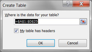 Excel still displays the dialog as shown below, but the dimensions of the data table defaults to the selected rectangle.  Be sure to check the checkbox if your table has headers as mine does so that these headers become the column names.

After clicking OK to create the table, define the sort for the table rows.  Since the table should still be selected, simple choose Sort from the Data ribbon to display the dialog shown below.  To sort on more than one column you must define the order in which you are sorting the columns from the top of the list downward.

In this example, I first sort on the Year column.  This column can be a simple sort on the column values from the smallest to the largest.  Remember that you when you sort years save as text, the order is the same as sorting years saved as numbers.

Within each  year, I next want to sort by month.  Again I will select to sort on Values.  However, simply sorting alphabetically does not satisfy the sort requirement as April falls before January.  However, I posted a blog entry a few weeks ago named: “Create Your Own Custom List for Sorting Pivot Rows and Columns” to show how to define custom text lists in which to sort by.  It just so happened that we created a custom list for the month names in a year.  We can reuse that list here to make sure that the months are sorted correctly within each year.  To do this, select Custom List from the Order dropdown.

Then select the custom list you want to use.  If you do not have a custom list yet for the months of the year, now would be a great time to create one.  The following figure shows the selection of the full month names custom list.

We are now ready to publish the Excel spreadsheet to our site, …almost.  First we have to make sure that Excel Services is turned on and is set to trust the site where we will deploy our spreadsheet.  If you do not have rights to Central Administrator, you may need to find your SharePoint administrator and ask him/her for some help to perform the next few steps.

From Central Administrator’s main page, locate the Application Management group and select the option Manage service applications as shown in the figure to the right.

From the page that lists all the service applications, make sure that the Excel Services application has been started as shown to the right of the name.  If not, start it now.

Next click on the title: Excel Services Application.  This allows you to define which sites support Excel services and lets you set various properties for each site.  Note, you must do this by site, not by individual Excel application.

First click on Trusted File Locations.  Central Administrator first shows all the file locations (sites) where Excel Services is currently enabled to support Excel spreadsheets.

If you do not see your site in the current list of trusted file locations, click on the link: Add Trusted File Location to add it.

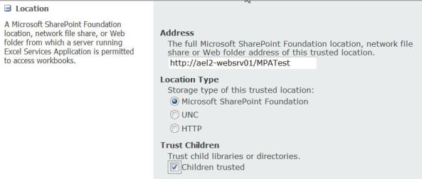
First you must define the site address.  The site address is the root to the site, not to the specific site library or page where you will be storing or using the Excel spreadsheet.  You probably also want to click the option to trust child libraries and directories as shown in the following figure.

There are other options on this page that you can set. While I will not go through all of these options here, you may want to look at a few of the settings such as:

Workbook Calculation Mode	Set to Automatic
Allow External Data	Trusted data connection libraries and embedded

When you have finished defining the Trusted File Location, return to your Excel spreadsheet and begin publishing it to the trusted site.  From the BackOffice area, select Save & Send to open the available save options.  In the first column click the Save to SharePoint option.  This displays Recent Locations where you may have previously published Excel spreadsheets (if any) and a list of other locations.  Note that the last option in the Locations group lets you browse for a new location.  If you have never published a spreadsheet to the site you want to use, you can either browse to it, or select the Save As button where you can enter the information.

The Save As button displays a standard Windows Save dialog which prompts you for a name and a data type.  If you know the fully qualified name including the site, library and filename, you can enter them all at once in the dialog box and click Save.  However, you can also enter just the name of the site as shown in the following figure.

If you enter the name of the site as the File name, the dialog retrieves from your SharePoint site a list of the libraries available as well as the names of any sites or workspaces embedded within the current site.  You can select the library where you want to store the Excel file by double clicking its name or by single clicking the name and then clicking the Open button.

However, before you click on Open, look at some of the other option available to you when you publish an Excel spreadsheet.  First, you see two checkboxes.  The first tells SharePoint that you want to open this Excel spreadsheet in the browser and not just use SharePoint to save the file.  The second checkbox saves a thumbnail image of the first spreadsheet page that can be used to help identify your spreadsheet from a group of spreadsheets.

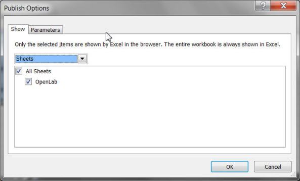
More interesting is the Publish Options button.  When you click this button, you get a dialog with two tabs: Show and Parameters.

The Show tab lets you define what part of the spreadsheet you want to publish.  By default Excel assumes that you want to publish the entire workbook.  You can select the spreadsheets to publish using the Sheets option and the list of available sheets.  You can also use the dropdown to select named ranges to publish.  In this simple example, I will publish all of the worksheets in the workbook.

The second tab lets you define parameters for the spreadsheet.  By default, a spreadsheet published to SharePoint cannot be edited.  However, you can define parameters.  These are nothing more than named cells that serve as the data source for other calculations in the spreadsheet.  For example, you might have a cell that defines the interest rate for a spreadsheet used to calculate the month by month mortgage payments, interest, and principal.  Each times you change the interest rate; you might want to see the effect on the amount of your monthly payment that goes toward interest and principal.  By defining this named cell as a parameter, you can provide interactivity in the spreadsheet for the user.  Note however, that each parameter must reference a single cell.  You cannot define a range of cells with a single parameter reference.  When you are done setting your publishing options, click OK for the dialog and Save to begin the actual publishing process.  (Note, only after you have selected a library will the button say Save instead of Open.)

After you have published your spreadsheet, open a page where you want to use the Chart web part.  If you want, add an Excel Web Access web part from the Business Data categories as shown in the following figure to display the Excel spreadsheet.  However, this step is not necessary if all you want to do is to publish the chart.

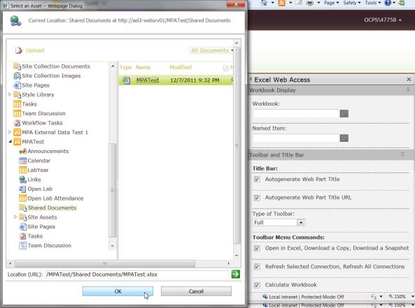
If you do want to display the spreadsheet, open the Excel Web Access’ tool pane and select the Excel Spreadsheet from the library where you published it.  You can enter the full URL of the Excel spreadsheet, but it is more likely that you will click the button to the right of the URL name field to open a dialog that lets you browse to the file.  The figure below shows the Excel Web Part’s tool pane to the right of the image while the browse dialog to find the Excel spreadsheet is on the left.

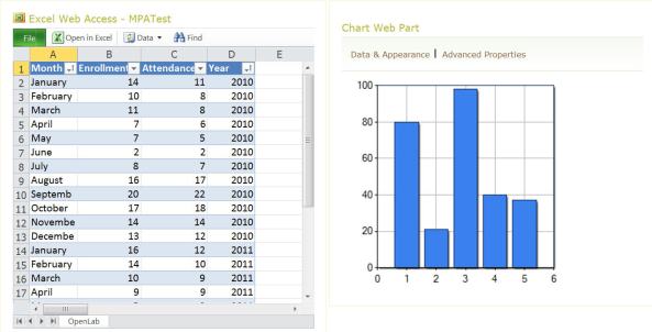
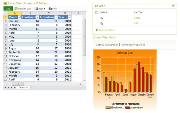
As shown on the left side of the following figure, the Excel Web Access web part displays the spreadsheet exactly as it appears in the Excel spreadsheet itself.  But what we want to show here is the data from the Excel spreadsheet in a Chart web part.  Therefore the Chart web part has been placed to the right of the Excel Web Access web part to make it easy for the user to look at the actual data associated with the chart.

In the last 3 posts in this series on the Chart Web part, we explored the Data & Appearance options that let you define the type of chart, and much of the formatting of the chart and its components.  When you click the Data & Appearance link, you will see the following option choices.

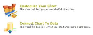
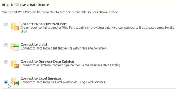
I am going to pick up the process after customizing the chart’s visual aspects by clicking on the link Connect Chart to Data.  In the screen shown in the following figure, choose the data source for the chart.  We previously covered the first three options.  This time, select the fourth option: Connect to Excel Services.

The second step of defining the data source requests information about the Excel Services Connection as shown below.  Unfortunately, none of the three text fields support dropdowns or browse buttons to help fill in these fields.  That makes this screen one of the hardest screens to complete so far.  The first text box however, should already have a default value in it.  Do not change this default value.  It should be correct.

The second text box is the path to the Excel Workbook.  This field is a tricky one to define.  Many users are familiar with the concept of right clicking on a document in a library to get a shortcut to that document.  However, sometimes the link that is provided is not a link to the document directly, but a link to a viewer application that then opens and displays the document.  The following link is an example:

http://ael2-websrv01/MPATest/_layouts/xlviewer.aspx?id=/MPATest/
Shared%20Documents/MPATest.xlsx&Source=http%3A%2F%2Fael2%2Dwebsrv01%2F
MPATest%2FShared%2520Documents%2FForms%2FAllItems%2Easpx&DefaultItemOpen=1
&DefaultItemOpen=1

Such is the case of Excel worksheets published to be opened in the browser.  You want to make sure that the link provided includes only the URL of the site, the library in which the worksheet is stored and the worksheet name ending with .xlsx.  Anything else will cause the connection to fail.  Therefore, in my case, the Excel Workbook Path was:

http://ael2-websrv01/MPATest/Shared%20Documents/MPATest.xlsx

The third text box can either be a range representing the data using the standard column and row format or if you defined a named range for the entire table in the original spreadsheet before publishing it, you can simply enter that name here.  Notice also that if you use the column and row designation, you must include the name of the worksheet, even if you only have one worksheet in the published workbook.  By default this name is Sheet1.  However, if you renamed it in your workbook, you must use the name that appears on the tab at the bottom of the current worksheet.  For example, in my case the worksheet tab name is: OpenLab.

Finally, if your worksheet includes column names in the first row, you must click the checkbox to tell the Chart web part that the range specified includes column names in the first row.  Should you just define your data range without the column name row?  No, because when you set up your chart, you may find it more meaningful to reference your data series by their column names.

In the third step of defining your chart’s data connection, you can define a filter.  Here you can select the column from the Excel Spreadsheet such as Year, which has a type of String, and specify a default value of 2010 as shown in the following figure.  The column that you provide here can be connected with a custom SharePoint list as described at the top of this post to filter the data in the chart.

 

In step 4, you can define for each series in the chart which columns you want to plot along with the series type and some other parameters that we have seen before in the prior posts and will not be reviewed in detail here.

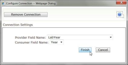
After defining the data source for the Chart, you can create the connection between a custom SharePoint list such as LabYear shown below by sending the selected row of data to the Chart web part.

The actual connection must then be established between the provider field in LabYear named LabYear and the Consumer Field Name in the Chart web part named Year (remember the filter parameter we just set). 

When you click Finish, you can control which year of data the Chart web part displays by selecting the year from the LabYear list as shown in the following and final figure of this post.

This concludes my 4-part mini-tour of the Chart Web Part and the different ways to provide data to the chart.  I hope you learned how easy it is to add charts to your SharePoint pages.  As you can see in this last figure, a picture can always make it easier to interpret a set of data.